Chionotech

Implementing the Gauss-Newton Algorithm for Sphere Fitting (3 of 3)

Posted on September 15, 2012 by Rolfe Schmidt

The first post in this series made it clear that the major computational and storage costs to implementing the Gauss-Newton algorithm come in computing the matrices ${\mathbf{J}_{\bar{\beta}}^{\top}\mathbf{J}_{\bar{\beta}}}$ and ${\mathbf{J}_{\bar{\beta}}^{\top}\vec{\mathbf{r}}}$ . By carefully avoiding materialization of the Jacobian matrix and the residual vector, the second post gave us a viable sphere fitting algorithm that can be used to calibrate common MEMS accelerometers (e.g. ADXL335, ADXL345) and magnetometers (e.g. HMC5843). This algorithm still requires multiple passes over the observation data, and that is only possible if all of those observations are stored somewhere; its space complexity is ${O(N)}$ where ${N}$ is the number of observations.

In this post we will see how to eliminate that requirement and perform the Gauss-Newton algorithm in a one-pass streaming algorithm with space complexity effectively ${O(1)}$ .

1. The heart of the matter

Notice that we can rewrite the ${0,0}$ entry of ${\mathbf{J}_{\bar{\beta}}^{\top}\mathbf{J}_{\bar{\beta}}}$ as follows

$\displaystyle \begin{array}{rcl} [\mathbf{J}_{\bar{\beta}}^{\top}\mathbf{J}_{\bar{\beta}}]_{00} &=& \sum_{i=0}^{N-1} 4\frac{(x_{i0} - \beta_{0})^2}{\beta_{3}^4} \\ &=& \frac{4}{\beta_{3}^4}\left[ \sum_{i=0}^{N-1} x_{i0}^2 - 2\beta_0\sum_{i=0}^{N-1}x_{i0} + \sum_{i=0}^{N-1}\beta_0^2\right] \\ &=& \frac{4}{\beta_3^4}\sum_{i=0}^{N-1}x_{i0}^2 - \frac{8\beta_0}{\beta_3^4}\sum_{i=0}^{N-1}x_{i0} + \frac{4\beta_0^2}{\beta_3^4}N \end{array}$

So if we know ${\sum_{i=0}^{N-1}x_{i0}^2}$ , ${\sum_{i=0}^{N-1}x_{i0}}$ , and ${N}$ , then we can compute the matrix entry for arbitrary ${\bar{\beta}}$ . We can scan the data once, compute these three numbers and then just use the formula above to compute the matrix entry while iterating through the Gauss-Newton algorithm. Once these numbers are computed, there is never a need to look at the data again.

A similar situation arises for all og the matrix entries. Before proceeding, let’s introduce some new notation that will make the sequel easier to follow, easier to code, and easier to generalize.

2. Notation

To think clearly about the calculations here, we need to stop thinking about 3-vectors and start thinking about ${N}$ -vectors. We will build on the notation introduced in post 1 of this series and define three new ${N}$ -vectors. For an axis ${j \in \{0,1,2\}}$ define

$\displaystyle \vec{\mathbf{x}}_{\bullet j} = \left[ \begin{array}{c} x_{0j} \\ x_{1j} \\ \vdots \\ x_{(N-1)j}\end{array} \right]$

This is the ${N}$ -vector of all observations for that axis. Next define

$\displaystyle \vec{\mathbf{x^2}}_{\bullet j} = \left[ \begin{array}{c} x_{0j}^2 \\ x_{1j}^2 \\ \vdots \\ x_{(N-1)j}^2\end{array} \right]$

This is the ${N}$ -vector of the squares of the observations along this axis. Finally, it will be convenient to use a vector of all ones:

$\displaystyle \vec{\mathbf{1}} = \left[ \begin{array}{c}1 \\ 1 \\ \vdots \\ 1 \end{array} \right]$

For any pair of ${N}$ -vectors ${\vec{\mathbf{x}}}$ , ${\vec{\mathbf{y}}}$ , we define the inner product as usual

$\displaystyle \langle \vec{\mathbf{x}}, \vec{\mathbf{y}} \rangle = \sum_{i=0}^{N-1} x_i y_i$

With this notation, we can rewrite the formula in the last section as

$\displaystyle \left[\mathbf{J}_{\bar{\beta}}^{\top}\mathbf{J}_{\bar{\beta}}\right]_{00} = \frac{4}{\beta_3^4}\left( \langle \vec{\mathbf{x}}_{\bullet 0}, \vec{\mathbf{x}}_{\bullet 0} \rangle - 2\beta_0\langle \vec{\mathbf{x}}_{\bullet 0}, \vec{\mathbf{1}} \rangle +\beta_0^2 N\right)$

3. Rewriting the matrix entry formulas

We will rewrite each of the formulas derived in post 2 in terms of these ${N}$ -vectors. It is a worthwhile exercise to verify these.

For ${j,k < 3}$

for ${j < 3 \leq k}$

and for ${ 3 \leq j,k}$

$\displaystyle \begin{array}{rcl} \left[\mathbf{J}_{\bar{\beta}}^{\top}\mathbf{J}_{\bar{\beta}}\right]_{jk} &=& \left[\mathbf{J}_{\bar{\beta}}^{\top}\mathbf{J}_{\bar{\beta}}\right]_{kj} \\ &=& \sum_{i=0}^{N-1} 4\frac{(x_{i(j-3)} - \beta_{(j-3)})^2(x_{i(k-3)} - \beta_{(k-3)})^2}{\beta_{j}^3\beta_{k}^3} \\ &=& \frac{4}{\beta_{j}^3\beta_{k}^3}\left( \langle \vec{\mathbf{x^2}}_{\bullet ( j-3)}, \vec{\mathbf{x^2}}_{\bullet (k-3)} \rangle -2 \beta_{(k-3)}\langle \vec{\mathbf{x^2}}_{\bullet (j-3)},\vec{\mathbf{x}}_{\bullet (k-3)} \rangle \right. \\ && \qquad+ \beta_{(k-3)}^2 \langle\vec{\mathbf{x^2}}_{\bullet (j-3)}, \vec{\mathbf{1}} \rangle -2\beta_{(j-3)}\langle \vec{\mathbf{x}}_{\bullet (j-3)}, \vec{\mathbf{x^2}}_{\bullet (k-3)} \rangle \\ & & \qquad + 4\beta_{(j-3)}\beta_{(k-3)}\langle \vec{\mathbf{x}}_{\bullet (j -3)},\vec{\mathbf{x}}_{\bullet (k-3)} \rangle - 2\beta_{(j-3)}\beta_{(k-3)}^2 \langle \vec{\mathbf{x}}_{\bullet (j-3)}, \vec{\mathbf{1}}\rangle \\ & & \left. \qquad + \beta_{(j-3)}^2 \langle\vec{\mathbf{1}}, \vec{\mathbf{x^2}}_{\bullet (k-3)} \rangle - 2\beta_{(j-3)}^2\beta_{(k-3)}\langle \vec{\mathbf{1}}, \vec{\mathbf{x}}_{\bullet (k-3)}\rangle - \beta_{(j-3)}^2\beta_{(k-3)}^2 N \right) \end{array}$

To we write similar expressions for the entries of ${\mathbf{J}_{\bar{\beta}}^{\top}\vec{\mathbf{r}}}$ , note that

$\displaystyle \vec{\mathbf{r}} = \vec{\mathbf{1}} - \sum_{j=0,1,2}\frac{1}{\beta_{3+j}^2}(\vec{\mathbf{x^2}}_{\bullet j} - 2\beta_j\vec{\mathbf{x}}_{\bullet k} + \beta_j^2\vec{\mathbf{1}})$

So for ${j < 3}$

$\displaystyle \begin{array}{rcl} \left[\mathbf{J}_{\bar{\beta}}^{\top}\vec{\mathbf{r}}\right]_{j} &=& \sum_{i=0}^{N-1}2\frac{x_{ij} - \beta_{j}}{\beta_{3+j}^2} \left( 1 - \sum_{k=0,1,2} \frac{(x_{ik} - \beta_{k})^2}{\beta_{3+k}^2} \right) \\ &=& \frac{2}{\beta_{3+j}^2} \left(\langle \vec{\mathbf{x}}_{\bullet j}, \vec{\mathbf{1}} \rangle - \sum_{k=1,2,3} \left(\langle \vec{\mathbf{x}}_{\bullet j}, \vec{\mathbf{x^2}}_{\bullet k} \rangle - 2\beta_k\langle \vec{\mathbf{x}}_{\bullet j}, \vec{\mathbf{x}}_{\bullet k} \rangle + \beta_k^2 \langle \vec{\mathbf{x}}_{\bullet j}, \vec{\mathbf{1}} \rangle\right) \right. \\ && \qquad \left. - \beta_j N + \beta_j\sum_{k=1,2,3} \left(\langle \vec{\mathbf{1}}, \vec{\mathbf{x^2}}_{\bullet k} \rangle - 2\beta_k\langle \vec{\mathbf{1}}, \vec{\mathbf{x}}_{\bullet k} \rangle + \beta_k^2 N\right) \right) \end{array}$

and for ${j \geq 3}$

$\displaystyle \begin{array}{rcl} \left[\mathbf{J}_{\bar{\beta}}^{\top}\vec{\mathbf{r}}\right]_{j} &=& \sum_{i=0}^{N-1}2\frac{(x_{i(j-3)} - \beta_{j-3})^2}{\beta_{j}^3} \left( 1 - \sum_{k=0,1,2} \frac{(x_{ik} - \beta_{k})^2}{\beta_{3+k}^2} \right) \\ &=& \frac{2}{\beta_{j}^3} \left(\langle \vec{\mathbf{x^2}}_{\bullet (j-3)}, \vec{\mathbf{1}} \rangle - \sum_{k=1,2,3} \left(\langle \vec{\mathbf{x^2}}_{\bullet (j -3)}, \vec{\mathbf{x^2}}_{\bullet k} \rangle - 2\beta_k\langle \vec{\mathbf{x^2}}_{\bullet (j-3)}, \vec{\mathbf{x}}_{\bullet k} \rangle + \beta_k^2 \langle \vec{\mathbf{x^2}}_{\bullet (j-3)}, \vec{\mathbf{1}} \rangle\right) \right. \\ && \qquad -2\beta_{(j-3)}\langle \vec{\mathbf{x}}_{\bullet (j-3)}, \vec{\mathbf{1}} \rangle + 2\beta_{(j-3)} \sum_{k=1,2,3} \left(\langle \vec{\mathbf{x}}_{\bullet (j-3)}, \vec{\mathbf{x^2}}_{\bullet k} \rangle - 2\beta_k\langle \vec{\mathbf{x}}_{\bullet (j-3)}, \vec{\mathbf{x}}_{\bullet k} \rangle + \beta_k^2 \langle \vec{\mathbf{x}}_{\bullet (j-3)}, \vec{\mathbf{1}} \rangle\right) \\ && \qquad \left. + \beta_{(j-3)}^2 N - \beta_{(j-3)}^2\sum_{k=1,2,3} \left(\langle \vec{\mathbf{1}}, \vec{\mathbf{x^2}}_{\bullet k} \rangle - 2\beta_k\langle \vec{\mathbf{1}}, \vec{\mathbf{x}}_{\bullet k} \rangle + \beta_k^2 N\right) \right) \end{array}$

These expressions may look tedious, but they are just straightforward algebra. If we scan the observation data ${\mathbf{x}_i}$ and compute the following statistics for all ${j,k \in \{0,1,2\}}$ we will have all of the information we need to compute our matrix entries:

$\displaystyle \begin{array}{|l| l| } \hline \text{Array} & \text{Size} \\ \hline \vspace{2pt} \langle \vec{\mathbf{x}}_{\bullet j}, \vec{\mathbf{1}} \rangle & 3 \\ \langle \vec{\mathbf{x^2}}_{\bullet j}, \vec{\mathbf{1}} \rangle & 3 \\ \langle \vec{\mathbf{x}}_{\bullet j}, \vec{\mathbf{x}}_{\bullet k} \rangle & 6 \text{ (symmetric)} \\ \langle \vec{\mathbf{x^2}}_{\bullet j}, \vec{\mathbf{x}}_{\bullet k} \rangle & 9\\ \langle \vec{\mathbf{x^2}}_{\bullet j}, \vec{\mathbf{x^2}}_{\bullet k} \rangle & 6 \text{ (symmetric)}\\ \hline \end{array}$

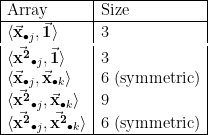
In fact, the situation is even better. Notice that

$\displaystyle \langle \vec{\mathbf{x}}_{\bullet j}, \vec{\mathbf{x}}_{\bullet j} \rangle = \langle \vec{\mathbf{x^2}}_{\bullet j}, \vec{\mathbf{1}} \rangle$

So we do not need to store ${\langle \vec{\mathbf{x^2}}_{\bullet j}, \vec{\mathbf{1}} \rangle}$ . Also the arrays ${\langle \vec{\mathbf{x}}_{\bullet j}, \vec{\mathbf{x}}_{\bullet k} \rangle}$ and ${\langle \vec{\mathbf{x^2}}_{\bullet j}, \vec{\mathbf{x^2}}_{\bullet k} \rangle}$ are symmetric, allowing us to store just 6 of the 9 entries. Altogether, we need to store 24 numbers. Of course we also need to store ${N}$ , the number of observations, for a total of 25.

4. Putting it into code

Implementing this is straightforward even if it demands a bit of care. To see this implemented, look at the file BestSphereGaussNewtonCalibrator.cpp in muCSense. Here is a quick overview of what to look for.

The arrays of statistics are private members of the BestSphereGaussNewtonCalibrator class and are declared in BestSphereGaussNewtonCalibrator.h

The statistics are all accumulated in the function in the method BestSphereGaussNewtonCalibrator::update (BestSphereGaussNewtonCalibrator.cpp).
The calibration matrices are computed in the function in the method BestSphereGaussNewtonCalibrator::computeGNMatrices (BestSphereGaussNewtonCalibrator.cpp).In muCSense this sphere fitting procedure is used to calibrate “spherical sensors” such as magnetometers and accelerometers. At present, the library specifically supports the inertial sensors on SparkFun’s 9DoF Sensor Stick: the ADXL 345 accelerometer, HMC 5843 magnetometer, and the ITG 3200 gyroscope. To use this code to calibrate a different accelerometer or magnetometer, you just need to define a new subclass of Sensor — see ADXL345.h/ADXL345.cpp for an example — then follow this example sketch.

5. What’s next.

The code in muCSense works, but needs to be optimized. As it is, a simple sketch using this calibration algorithm takes up 20K of the 32K available on an Arduino Uno. The sums and products have a clear structure that I have not attempted to exploit at all. Using this structure should allow a valuable reduction in compiled code size. I will work on this, but would love to hear from anyone else who has some ideas.

It is interesting to note that this algorithm has a clear generalization to any residual function which is a polynomial of the observation vector. It works for higher dimensional observations and for higher degree polynomials. In particular, it can be adapted to handle linear maps with shear, something I plan to implement soon. The process I walked through here should be abstracted to build a system that takes a polynomial residual function as input and determines the statistics and computations needed in the background, optimizing the tedious arithmetic and saving us from writing this sort of code.

Posted in Mathematics | Tagged Accelerometer, ADXL335, ADXL345, Arduino, Calibration, Gauss–Newton algorithm, HMC5843, Magnetometer, muCSense, Sensor, Statistics | 4 Comments

Implementing the Gauss-Newton Algorithm for Sphere Fitting (2 of 3)

Posted on September 8, 2012 by Rolfe Schmidt

I sketched a naïve implementation of the Gauss-Newton algorithm for sphere fitting, and provided an implementation in Octave. While it works fine on a laptop, it uses far too much memory to handle more than a handful of calibration samples on a microcontroller.

What took up all of that memory? The matrix ${\mathbf{J}_{\bar{\beta}}}$ , the vector ${\vec{\mathbf{r}}}$ , and the set of observations ${\mathbf{x}_i}$ .

It turns out that we don’t really need to keep any of these around. In this post I’ll describe how to implement the algorithm without materializing ${\mathbf{J}_{\bar{\beta}}}$ and ${\vec{\mathbf{r}}}$ . This will reduce the memory footprint enough to make a practical algorithm that can handle ~100 observations. This is the algorithm used in the accelerometer calibration sketch I posted last year.

In the next post, I’ll show how to accumulate 25 statistics about the observations that have all of the information we need to run Gauss-Newton in constant space and time.

Let’s start by getting rid of the big arrays of statistics. Continue reading →

Posted in Mathematics | Tagged Accelerometer, ADXL335, Arduino, Calibration, Gauss–Newton algorithm, Magnetometer, muCSense, Statistics | 2 Comments

Implementing the Gauss-Newton Algorithm for Sphere Fitting (1 of 3)

Posted on September 1, 2012 by Rolfe Schmidt

In some calibration strategies we encounter a sphere fitting problem: we need to find the map that does the best job sending the observed data to a unit sphere. This simple problem statement leaves two critical questions unanswered.

What family of maps are we picking from?
How do measure “best”?

I’ll outline a wealth of options we have in answering these questions in later posts. This article will specify reasonable answers to these questions, use those answers to pose a clear problem, then describe an algorithm to solve the problem.

The naïve algorithm presented here is easy to implement but requires too much memory for many micro-controller applications. Some simple refinements give us a second algorithm that still requires space linear in the number of samples, but with a constant small enough to make it usable on an Arduino. Finally we observe that we can collect 25 summary statistics of our data and have all the information we need to carry out the Gauss-Newton algorithm, giving us a constant space, constant time streaming algorithm. These algorithms will be described in detail in later articles.

Although the focus here is on sphere fitting, the methods described, including the constant-space streaming algorithm, have straightforward (if tedious) extensions to very general polynomial mapping problems. Continue reading →

Posted in Mathematics | Tagged Accelerometer, Arduino, Calibration, Gauss–Newton algorithm, Magnetometer, muCSense, Statistics | 2 Comments

muCSense: Using Calibration

Posted on August 28, 2012 by Rolfe Schmidt

I just added some new code to the muCSense library to help calibrate accelerometers and magnetometers. I plan to use the framework to add calibrators for gyros and other sensors too.

In this post, I’ll walk through an example sketch that uses these new classes. I’ll dig into the internals in later posts.

The Circuit

This sketch assumes that you have connected a SparkFun Sensor Stick to an Arduino (I have an Arduino Uno), just as I described a while back. Here’s the diagram (after the jump):

Continue reading →

Posted in Electronics, How To | Tagged Accelerometer, ADXL345, Arduino, Calibration, HMC5843, ITG-3200, muCSense, Observer pattern, Sensor, SparkFun Sensor Stick | 3 Comments

muCSense: Introduction and Example

Posted on August 24, 2012 by Rolfe Schmidt

In my last post I walked through the steps you need to take to establish a simple connection with the three sensors on SparkFun’s 9DoF Sensor Stick. If you took those code snippets, dumped them into one file, and ran it on your Arduino…

you’d have a big mess.

It would work, but it would be awful to read, maintain, or upgrade. And what if you wanted to put some real logic in it? Maybe something that does more than dump raw readings to Serial?

And what happens when we get other sensors? We will usually be doing the same things:

Define device-specific constants, likely lifted from the datasheet.
Initialize.
Read data.
Calibrate.
Maybe tweak some device specific parameters, listen for interrupts, etc.

Everything but item 5 can be pretty well abstracted away, and we can encapsulate all of the device specific mess in classes that won’t clutter our code or namespaces. Doing this will leave us with code that is more robust, easier to use correctly, and easier to maintain.

That’s why I am writing muCSense. Continue reading →

Posted in Electronics, How To | Tagged ADXL345, Arduino, HMC5843, ITG-3200, muCSense, Programming, Sensor, SparkFun | 5 Comments

Connecting to Sparkfun’s 9DOF “Sensor Stick”: I2C access to ADXL345, ITG-3200, and HMC5843

Posted on February 10, 2012 by Rolfe Schmidt

[Update 24 Aug 2012: This post gives good detail about how to communicate with the sensors on the 9DoF Sensor Stick, but if you want a cleaner solution (that has been updated for Arduino 1.0), have a look at this post.]

Accelerometers are fun, but I want something more. So I picked up a “sensor stick” from Sparkfun.

Sparkfun’s 9DOF sensor stick. Image courtesy of Sparkfun Electronics is CC by NC-SA 3.0

It has an ADXL345 accelerometer (datasheet) , an ITG-3200 gyroscope (datasheet), and an HMC5843 magnetometer (datasheet). When still, the accelerometer can read the local gravitational field and the magnetometer can read the local magnetic field. As long as I’m not at a magnetic pole, this is enough to give me an external frame of reference and know exactly how my sensor is positioned in space. When the device is spinning, the gyro can help me separate translational acceleration from rotational acceleration as well as help me keep a running estimate of my sensor’s orientation even when I can’t trust the acceleration. A system that does this is called an Attitude and Heading Reference System [AHRS].

I’m just getting into the Mathematics of how to use all of this data, and it is going to be good fun. For today I’m going to talk about a much simpler problem: how do you connect to this board, initialize it, and read data from it. Continue reading →

Posted in Electronics, How To | Tagged Accelerometer, ADXL345, Arduino, Attitude and heading reference system, Gyro, HMC5843, I²C, ITG-3200, Magnetometer, Sensor | 41 Comments

Accelerometer Calibration IV.1: Implementing Gauss-Newton on an ATMEGA

Posted on October 24, 2011 by Rolfe Schmidt

This is the third post in a series.

Introduction
Simple Methods
Least-Squares and Gauss Newton
Implementing Gauss-Newton on an ATMEGA (this post)
Error Analysis
?

Quick Summary

This post is short on explanations, I just wanted to something a bit more useful out. We can implement the Gauss-Newton method directly on an Arduino using this sketch to drive a circuit with an ADXL 335 and two pushbuttons like this:

Two button circuit used to calibrate an ADXL335

Once the circuit is wired and the sketch is uploaded, open the serial monitor and move the thing around to 6 or more distinct positions. In each position push the button on pin 2, and hold it still for a second (or until you see the reading print out on the serial monitor. After you’ve collected at least 6 readings, push the button on pin 3 — this will perform the optimization and print your parameters.

See how I do it in this very fuzzy video:

Some details

In the last post we saw how we could use the Gauss-Newton method to use any set of sample reading from a still accelerometer to get an accurate calibration. The big problem was the tediousness. We took measurements on an arduino, sent it over the serial connection to a computer, ran scripts on the computer to compute calibration parameters, then reprogrammed the Arduino with the new parameters. Sure most of this could be automated, but it would still require a serial connection to a “real” computer with more than 1K of RAM.

To fix this, we need to implement Gauss-Newton directly on the arduino, but the ATMEGAs 1K to 2K memory limitation makes this challenging. We simply cannot store the big matrices used in the intermediate calculations of the Gauss-Newton method. To get around this, we do two things.

To reduce the number of data samples we need to store without losing too much information about the distribution of samples, we let the accelerometer sit in each position long enough to collect a few samples (I picked 32), then we average them and computed the variance.
We never materialize the large matrices, instead just compute the smaller matrices on the fly when they are needed.

There are a few other tricks I use to improve the data quality, and I’ll go over all of the details in the next post where I plan to walk through the code.

Even though it is handheld and held by a hand that had too much coffee, this process gives highly repeatable results. I performed this calibration 20 times and recorded the parameters produced. You can see the data in this spreadsheet. The summary is this: the zero-G parameters on each axis has standard deviations less than 0.03% and the sensitivity parameters all had standard deviations less than 0.2%. Accurate? Maybe 🙂 Repeatable? definitely.

On-Arduino Gauss-Newton Calibration Overall Grades: Accuracy – Great Easiness – Great

In the next post I’ll explain the details behind all of this, then move on to error analysis, saving parameters in EEPROM, and more.

Posted in Electronics, How To | Tagged Accelerometer, ADXL335, Arduino, Calibration, Gauss–Newton algorithm, Sensor, Statistics | 13 Comments

Accelerometer Calibration III: Improving Accuracy With Least-Squares and the Gauss-Newton Method

Posted on August 26, 2011 by Rolfe Schmidt

This is the third post in a series.

Introduction
Simple Methods
Least-Squares and Gauss Newton
Streaming Gauss-Newton on an ATMEGA
Error Analysis
?

In the last post we looked at some simple calibration methods and they didn’t seem to get us results that were better than the ones we got by just trusting the datasheet. There were two obvious problems:

Our calibration methods assumed we had placed our accelerometer in perfect axial alignment each time. We were, um, less than perfect.
We ignored the fact that there is noise in the sensor readings. Eyeballing it, this alone would give us about ~1% error.

We could address problem (1) by finding ways to place our device very carefully before taking measurements. We could address problem (2) by averaging our samples (and assuming that the average was a good estimate of the real values).

Instead, we will use some Mathematics to develop a calibration method that is robust to noise and is not dependent on careful sensor placement. This will give more accurate results even though it requires less care by the user. Continue reading →

Posted in Electronics | Tagged Accelerometer, ADXL335, Arduino, Calibration, Gauss–Newton algorithm, Sensor, Statistics | 18 Comments

Accelerometer Calibration II: Simple Methods

Posted on August 26, 2011 by Rolfe Schmidt

This is the second post in a series. It starts here.

Now let’s look at some of the simplest methods we can use to calibrate an accelerometer. By “simple” here I mean simple all the way through: easy to wire the circuit, easy to code, easy to understand, easy to use. Later we’ll see that these don’t always come as a package: fairly sophisticated software can make the users job even simpler than anything we see here.

The simple methods I will describe here all follow the same flow: the user carefully places the accelerometer in position, flips a switch to tell it to start recording data, flips the switch back to tell it to stop, then moves the accelerometer into a different position to start again. The differences all come down to deciding how many measurements to take and what to do with the numbers we get. Because of that, all of these methods can be performed using the same simple circuit.

Let’s build that before we go on. Continue reading →

Posted in Electronics | Tagged Accelerometer, ADXL335, Arduino, Calibration, Sensor | 3 Comments

Accelerometer Calibration I: Introduction

Posted on June 22, 2011 by Rolfe Schmidt

In my last post I described how to start reading data from an ADXL335 accelerometer with an Arduino and convert those voltage readings into standard units. I even showed some real data coming out of my device and when you looked at it, it was pretty clear that:

The data coming out were stable and repeatable
The conversion I used wasn’t right: the acceleration of gravity changed depending on the tilt of the accelerometer.

The problem is that I wasn’t really calibrating. I never took measurements from my device and compared them with known values. I just trusted the datasheet (which doesn’t promise anything precise, by the way). Even if the datasheet promised exact sensitivity, it doesn’t know how the sensor will be placed in the circuit. For example:

Is the soldering dodgy on any of the pins?
Is the sensor tilted in the device? (yep, it is off by a few degrees thanks to that dodgy soldering.)
Is everything on the circuit exactly the same downstream from the sensor pins?

Because the sensor readings are stable and repeatable, real calibration gives much better results. It just takes a bit more work. In this series of posts I’ll survey a few calibration methods starting with faith-based methods like reading datasheets, moving on to naïve but effective calibration, and finishing off with nonlinear least-squares based approaches that require a bit more Math.

Evaluating calibration methods

Before jumping in to the specific techniques, I want to say a few words about how I evaluate them. I have two basic metrics:

How accurate is the calibration?
How easy is it to perform the calibration?

To evaluate accuracy, I produced a standard data set with the accelerometer held fixed in 14 different known positions (approximately corresponding to the faces of a truncated cube). I use methods I’ll describe in another post to determine what the “true” accelerometer reading should be at each of these positions then compare that to the reading I get from whatever calibration method I am testing.

If I have such a great calibration method and can get the “true” values out of my device, why do I bother with other techniques? Well, for one I am curious about how good they are. But the real problem is that the best calibration method is not easy to perform: it involved 30 minutes of careful device placements, measurements, button pushing, and data recording. If it were possible to get an error on the order of 1% with less than 10 seconds of work wouldn’t you consider making that trade-off?

That is why I also evaluate how easy each calibration method is to perform. When I talk about ease of calibration, I am not talking about how easy it is to write the code. I’m giving you all the code anyway. All I care about is this:

How easy is it to get a device calibrated after it has been programmed?

If calibration takes thirty minutes of futzing and special equipment, I’ll say the easiness is bad. If it just takes a button press and 10 seconds of moving the device around I’ll say it is pretty good. If it doesn’t require anything at all, then it is great.

Sure, you can automate a tedious and error-prone calibration process if the results are so much better it makes it worthwhile, but that is not much help for DIYers or prototyping. Also, for the skiing devices I’m building I want to have a way to recalibrate them in the field when I reconfigure them or even just because the temperature changed.

So every calibration method I describe will get two grades: one for accuracy and one for easiness. In the end, we will see that there are some methods that get good marks in both categories.